A Primer to Bayes' Classifier

09 Jan 2020

The Bayes’ classifier is a powerful tool in any machine learning practitioner’s arsenal. It’s a generative model and by exploiting Bayes’ rule can be used for classification. In this article we’ll first understand Bayes’ Rule as applied to a supervised classification problem following which we’ll program an algorithm to classify digits using a Naive Bayes’ classifier.

Conditional Probability

Consider two random variables $X, Y$, the conditional probability is given by, $P(X \vert Y) = \frac{P(X, Y)}{P(Y)}$. The idea encapsulated by this equation is extremely useful can be understood through a simple example. If $X$ represents certain attributes of a vehicle (like speed, chassis type, etc.) and $Y$ represents the type of vehicle (eg. a bike, a sedan, a sports car, a truck, etc.) then $P(X \vert Y)$ denotes the probability of the attributes (or features) of a vehicle being $X$ given the vehicle type $Y$.

Within the context of digit classification, $X$ represents the features which encode information about the digits while $Y \in \{0,1,…,9\}$ represents the class of the digit.

Bayes’ Rule

Bayes’ Rule states that $P(Y \vert X) = \frac{P(X \vert Y)P(Y)}{P(X)}$. Using our example, this means we can determine the probabilty of a given vehicle being a bike, a car or a truck given its features by first computing the likelihood of observing the features ($X$) of a given vehicle type and the marginal probabilities of those vehicles and their attributes.

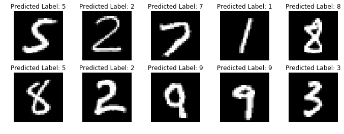
Let’s consider the example for digit classification in more detail. Let’s assume we have a dataset handy (like MNIST [1]). Every digit in the dataset is written in a certain manner. Using the information about the curvature, number of straight lines or even their intersections we can determine the representation of the digit. If we see a new digit we can use the information gleaned from analysing the MNIST dataset to inform our decision about the type of digit. In other words, we can generate a probability distribution $P(Y \vert X)$ which tells us which digit seems most likely from the features we’ve observed. Here, $P(Y)$ would be the marginal probability of observing digit $Y$ in the MNIST dataset. $P(X \vert Y)$, the likelihood of observing some features $X$ given the digit $Y$, for instance the probablity of seeing a large curvature if our digit was $Y = 1$ (which would be small since 1 is usually written as a vertical line). $P(x)$ is the marginal probability of the features $X$ and works as a normalizing constant computed using $P(X) = \sum_i P(X \vert Y=i) P(Y=i)$.

Naive Bayes’ Assumption

The discussion about features brings us to the Naive Bayes’ assumption. Normally, $X$ comprises several features and these features are not necessarily independent. For instance, the area of the hole in a zero and the thickness of its strokes. As a result in order to compute $P(X \vert Y)$ we can break it down as,

$P(X \vert Y) = P(X_n \vert Y, X_1,...,X_{n-1})P(X_{n-1} \vert Y, X_1,...,X_{n-2})...P(X_1 \vert Y),$

for $n$ features. However, this makes the computation significantly more complex since it’s generally not easy to determine the influence of one feature on another. This is where the Naive Bayes’ assumnption comes in handy.

Naive Bayes’ assumption is that if we’re given the class $Y$, then the features are independent of each other. This allows us to rewrite the above as,

$P(X \vert Y) = P(X_n \vert Y)P(X_{n-1} \vert Y)...P(X_1 \vert Y) = \Pi_j P(X_j \vert Y),$

While this may not be true in majority of the cases it works surprisingly well in practice, with the added benefit of making computation of the likelihood easier.

Computing the Likelihood $P(X \vert Y)$ and Prior $P(Y)$

As discussed earlier, $P(Y)$ represents the marginal distribution of $Y$. In Bayesian Inference, $P(Y)$ is referred to as the prior and it encapsulates our initial beliefs about the data. For digit classification, it represents our prior beliefs in encountering a particular digit. For instance, if we had an equal number of images for all digits in our dataset, each digit would be equally likely, thus $P(Y=0) = P(Y=1) = … = P(Y=9)$.

Armed with the Naive Bayes’ assumption we can compute the likelihood from the data that is available to us. The attributes $X$ that describe our data can be computed using several methodologies. For our example, we’ll compare two approaches - features based on pixel intensity and features based on histogram of oriented gradients.

Computing the Posterior $P(Y \vert X)$

In order to compute the posterior, $P(Y \vert X)$, we require one additional piece, $P(X)$. However, since $P(X)$ is a normalizing constant, $P(Y \vert X) \propto P(X \vert Y)P(Y)$. Thus for a class $Y=i$, our posterior would be proportional to $P(Y=i)\Pi_j P(X_j \vert Y=i)$. Since we require the class which maximizes the posterior $P(Y \vert X)$, we can make use of Maximum-A-Posteriori estimation [2] to determine the likelihood and prior. Thus, our required result will be given by,

$\hat{y} = \text{argmax}_{y \in Y} P(y)\Pi_j P(X_j \vert y)$

Generally, multiplication of probabilities can lead to numerical instabilities during computation so we work with the logarithm, which gives us,

$\hat{y} = \text{argmax}_{y \in Y} \bigg[\log(P(y)) + \sum_j \log(P(X_j \vert y))\bigg]$

Maximizing this is the same as maximing the preceding equation since the logarithm is a monotonically increasing function.

Digit Classification using Binarized Pixel Intensities

For classifying digits using their pixel instensities let’s first quantize their values. For simplicity, we’ll binarize the image so we’ll have only two quantization levels - 0 and 1. We can choose an appropriate theshold to achieve this, here we’ll use 127. Since a pixel intensity can take only two values {0, 1}, we can model their distribution as a bernoulli random variable. For each pixel $x$ in the image, we have $P(X=x \vert Y) = p^x(1-p)^{1-x}$. We can then write the loglikelihood as,

$\log P(X \vert Y) = \sum_j \log P(X_j \vert Y) = \sum_j x\log p + (1-x)\log(1-p)$

Accordingly, the class can be computed from the posterior by,

$\hat{y} = \arg\max_{y \in Y}\bigg[\log P(Y) + \sum_j x\log p + (1-x)\log(1-p)\bigg]$

Although, you’ll notice we can also use the likelihood instead of the loglikelihood as done in the program below.

  def get_binomial_parameters(X, labels, NUM_DIGITS=10):
  digit_freq = np.empty((NUM_DIGITS), dtype=np.int32)
  pixel_freq_ones = np.empty((NUM_DIGITS, X.shape[1]),dtype=np.int32)
  
  # compute probability of each digit in train set
  digit_freq = np.bincount(labels)
  idx = np.insert(np.cumsum(digit_freq), 0, 0)
  
  # compute pixel probabilities
  for digit in range(0,NUM_DIGITS):
      pixel_freq_ones[digit,:] = np.sum(X[labels == digit], axis=0)
  
  pixel_freq_zeros = (np.reshape(digit_freq,(digit_freq.size,1)).T - pixel_freq_ones.T).T
  pixel_freq = np.stack((pixel_freq_zeros / digit_freq[:,None], pixel_freq_ones / digit_freq[:,None]), axis=-1)

  return [digit_freq / labels.size, pixel_freq]

If we desire the probabilities for the posterior then we can also compute the marginal $P(X)$ using the likelihood and marginal for $P(Y)$ using $P(X) = \sum_i P(X \vert Y=i)P(Y=i)$.

  # compute the likelihood
  image_stack = np.stack((inv_curr_image, curr_image), axis=-1)
  pixel_intensity = np.repeat(image_stack[np.newaxis], NUM_DIGITS, axis=0)
  likelihood = np.sum(np.multiply(p, pixel_intensity), axis=2)
      
  # compute marginal probability
  marginal = np.sum(np.prod(likelihood,axis=1) * prior)

Once we have all the required components we compute the posterior as,

  # compute posterior probabilities and get predicted label
  posterior[idx] = np.prod(likelihood,axis=1) * prior / (np.prod(marginal) + eps)
  label_predicted[idx] = np.argmax(posterior[idx])

Using this method the highest accuracy we obtain is approximately $84.34\%$

Digit Classification using Grayscale Pixel Intensities

Let’s perform this classification using a different set of features. We’ll make use of the original grayscale images. The MNIST dataset has 784 pixels in an image, each pixel comprises a feature. Since the actual intensity values in an image are defined on a continuous scale we can use a Gaussian probability distribution to model the likelihood. As an aside, from here on we’ll model the distribution of all features as jointly Gaussian. A Gaussian distribution is parameterized by its mean $\mu$ and covariance $\Sigma$ (or the variance $\sigma^2$ in the scalar case). If we have $n$ pixels in the image, we can write,

$P(X \vert Y) \sim \mathcal{N}(X; \mu, \Sigma) = \frac{1}{(2\pi)^\frac{n}{2} \vert \Sigma \vert^\frac{1}{2}} \exp{\bigg(-(x-\mu)^T \Sigma^{-1} (x-\mu)\bigg)}$

Now, using the Naive Bayes’ assumption the only non-zero entries in $\Sigma$ will be the diagonal elements which correspond to the variance of each feature. This along with the log-likelihood allows us to write,

$\begin{align*} \log P(X \vert Y) &= -\frac{n}{2}\log(2\pi) - \sum_j \log \sigma_j - \sum_j \frac{(x_j - \mu_j)^2}{\sigma_j^2}\\ &\propto - \sum_j \log \sigma_j - \sum_j \frac{(x_j - \mu_j)^2}{\sigma_j^2}\\ \end{align*}$

We can drop the constant term since it doesn’t factor into the optimization. Now we can compute the class as,

$\hat{y} = \arg\max_{y \in Y} \bigg[\log(P(y)) - \sum_j \log \sigma_j - \sum_j \frac{(x_j - \mu_j)^2}{\sigma_j^2}\bigg]$

Let’s see how we can program this. First, we’ll need the parameters of the Gaussian distribution from the training set.

def compute_parameters(X, labels, NUM_DIGITS, NUM_PIXELS):
  # compute mean and variance of training set for Gaussian Naive Bayes
  mu = np.zeros((NUM_DIGITS, NUM_PIXELS))
  var = np.zeros((NUM_DIGITS, NUM_PIXELS))

  for i in range(NUM_DIGITS):
    idxs = labels == i
    mu[i] = np.mean(X[idxs], axis=0)
    var[i] = np.mean((X[idxs] - mu[i])**2, axis=0)
  
  return mu, var

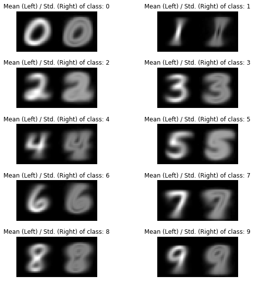
We can visualize the mean and standard deviation of each digit as seen in the figure below.

With the parameters and priors computed we can proceed to compute the likelihood for our test set in the following manner,

def gaussianNB(X, mu, var, prior, NUM_IMAGES, NUM_DIGITS):
  eps = 1e-8

  loglikelihood = np.zeros((NUM_IMAGES, NUM_DIGITS))
  logposterior = np.zeros((NUM_IMAGES, NUM_DIGITS))
  
  for i in range(NUM_DIGITS):
  # compute likelihood
    loglikelihood[:, i] = - (
      np.sum(np.log(var[i] + eps) / 2) \
      + 0.5 * np.sum((X - mu[i])**2 / (var[i] + eps), axis=1) / 2
    )
    # posterior
    logposterior[:, i] = np.log(prior[i]) + loglikelihood[:, i]

  # predict (argmax)
  labels_predicted = np.argmax(logposterior, axis=1)
  
  return labels_predicted

If we compute the accuracy of the using this naive approach it comes out to be roughly $49.89\%$. Why is it so low? An image has a large number of pixels and since pixel values don’t vary greatly over a small region, there is high correlation among them. This, in turn, can affect the prediction accuracy. To improve our prediction we could make use of Principal Component Analysis [3] to perform dimensionality reduction and use the features obtained through this process for classification. PCA essentially gives us the vectors along which we observe the maximum variance in the dataset. We can choose the components based on the magnitude of the singular values. We can implement this as below,

  def perform_PCA(X_train, X_test, n_components=70):
    pca = PCA(n_components=n_components, whiten=True, random_state=42)
    pca.fit(X_train)
    Xp_train = pca.transform(X_train)
    Xp_test = pca.transform(X_test)
    
    return Xp_train, Xp_test

With the new features, the accuracy on our test set turns out to be $82.95\%$, which is a drastic improvement over the naive methodology. Setting whiten to True yields vectors that are uncorrelated. What’s unique about jointly Gaussian features is that being uncorrelated implies independence and vice-versa, which allows us to exploit Naive Bayes’ to its fullest extent.

Digit Classification using Histogram of Oriented Gradients

Let’s try histogram of oriented gradients [4] to reduce the dimensionality of our feature space (note that computing HoG does not decorrelate the image features, it’s used to obtain feature descriptors. The reduced dimensionality is a by-product of this). We can use the OpenCV library to compute HoGs as,

  hog = cv2.HOGDescriptor((28, 28), (14, 14), (7, 7), (7, 7), 9)
  hog_features = hog.compute(image)

After obtaining the features, we need to compute the parameters of the density as discussed before and with that we’re done! Using HoG we get a classification accuracy of $91.83\%$, which is a significant improvement over the PCA technique.

[Github]