Bilateral Filter for Contrast Reduction

The bilateral filter is very versatile with several applications ranging from texture smoothing, to mesh construction to HDR imaging. In this project, we’ll first look at the motivation behind using the bilateral filter for contrast modification and subsequently implement a computationally efficient version for tone-mapping HDR images.

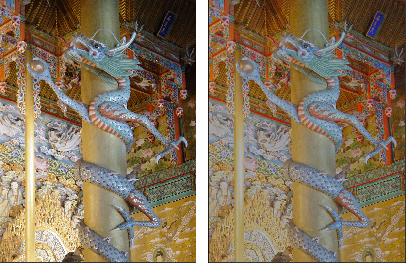
(Left to right) Original Image, Contrast Reduced Image

What is a bilateral filter?

A bilateral filter is commonly used for anisotropic image smoothing and noise reduction. In essence, it performs a non-linear filtering operation that treats different pixel locations differently depending upon their spatial coordinates and intensity values. Unlike averaging or median filters that result in a loss of important edge information, a bilateral filter is edge preserving.

We can compute the response of the bilateral filter at a given pixel $q$, which has a neighbourhood of pixels $\Omega$ in an image $I$ using the following equations,

\begin{equation} I_\text{filtered}(q) = \frac{1}{W_q} \sum_{p \in \Omega} I(p)f_r(|I(p) - I(q)|)f_s(|p - q|),
\end{equation} where, $W_q = \sum_{p \in \Omega}{f_r(|I(p) - I(q)|)f_s(|p - q|)}$

Here, $f_s$ is the spatial kernel and $f_r$ is the range kernel (defined over the set of intensities the image pixels can take). We see that the bilateral filter replaces the intensity of each pixel with a weighted average of intensity values from nearby pixels. This weight is represented by $W_q$. For computational simplicity both kernels are defined using Gaussians.

Why use a bilateral filter?

Image capturing, even under normal light conditions, can be difficult due to varying camera exposure levels. High Dynamic Range (HDR) images combine multiple images with different exposure levels to compute a radiance map. Since, most viewing devices cannot display HDR images they need to be tone-mapped. Tone-mapping maps the set of colors from a high dynamic range to a low dynamic range. The process is essentially a form of contrast reduction. This may introduce unwanted errors or eliminate finer details corresponding to edges. This is where a bilateral filter comes into picture. It can be used for contrast reduction while preserving edges.

An intuitive example

Credit: Frédo Durand, Julie Dorsey - Fast Bilateral Filtering for the Display of High-Dynamic-Range Images

Suppose we have an input image $I$ that looks like the noisy step function above. We first generate a Gaussian spatial kernel $f_s$ and a Gaussian range kernel. Now for a given pixel $q$ in $I$ we compute the response of range Gaussian to obtain the influence function $f_r$. To get the weight (net influence) of each pixel in $I$ on pixel $q$, we multiply the response of the spatial and range Gaussians to obtain the weight function.

What does this weight function do?

Let’s take a simple example. When the bilateral filter is centered, say, on a pixel on the higher intensity side of $I$, the function assumes values closer to $1$ for pixels on the same side, and values closer to $0$ for pixels on the dark side. In effect, with this weight function the filter replaces the pixel value by an average of the bright pixels in its vicinity, and ignores the dark pixels. Conversely, when the filter is centered on a dark pixel, the bright pixels are ignored instead. This is what helps preserve the edges in the filtering operation.

Once we have the weight function, we can use equation (1) to get our filtered output at $q$. Repeat this process for every pixel in $I$ and voila! We obtain the filtered (output) image.

Speeding up

The problem with a naive implementation of the bilateral filter is that it requires $\mathcal{O}(n^2)$ computation time for an image with n pixels. This quickly becomes a very expensive operation. [1] proposes two methods to speed up the computation - 1. view bilateral filtering as a convolution and perform it piecewise in the intensity domain and 2. downsample the image.

In order to see how convolution applies we look back at equation (1). If we assign $H(p) = I(p)f_r(|I(p) - I(q)|)$ then, $I_\text{filtered}(q) = \frac{1}{W_q} \sum_{p \in \Omega} H(p)f_s(|p - q|)$, which can be viewed as convolving a filter $f_s$ with a signal $H(p)$. The same argument holds for $W_q$ where our signal would become the response function of the range Gaussian. Now, we can discretize the intensity domain into fewer values and compute the filter response for each value.

To further improve the speed-up, the image can be downsampled without significant loss in quality. The images below show the output for downsampling factors of 2, 4, and 8. Notice how there isn’t a noticeable drop in the quailty of the results. On the other hand there’s a massive gain in performance. For an image of size 512x512 a decimation by a factor of 2 yielded a speed-up of almost 80%.

(Left to right) Original, Downsampled by 2, by 4, by 8

Implementation

First, we implement a 1D Gaussian. Note that we can always get a 2D Gaussian by taking the outer product of a 1D Gaussian with itself.

class Gaussian1D():
  # this is spatial gaussian
  def __init__(self, ksize, sigma):
    self.ksize = ksize # kernel size
    self.sigma = sigma  # standard deviation
    self.center = lambda x: x//2 if x//2 == 0 else (x-1)//2
    self.kernel = self.create_gaussian_kernel()

  def create_gaussian_kernel(self):
    gaussian_matrix = np.zeros((self.ksize,))
    values = np.linspace(0, self.ksize, self.ksize, endpoint=False)
    # distance from the desired pixel
    distance_squared = (values - self.center(self.ksize))**2
    # calulation of the gaussian function 
    self.kernel = 1 / (np.sqrt(2 * np.pi) * self.sigma) \
      * np.exp(-distance_squared / (2 * self.sigma**2))

    return self.kernel

With the Gaussian defined, we can now implement the algorithm as follows,

# for all the quatized intensity levels
for j in range(nb_segments):
  i_j = j * Idelta + Imin # get quantization intensity level

  # bilateral filtering for specific quantized intensity
  G_j = rkernel.apply(i_j) # apply the range Gaussian to quantized intensity
  K_j = cv2.sepFilter2D(G_j, ddepth=-1, kernelX=kernel_X, kernelY=kernel_Y) # kernelX and kernelY are gaussian kernels; 
  H_j = G_j * I
  H_star_j = cv2.sepFilter2D(H_j, ddepth=-1, kernelX=kernel_X, kernelY=kernel_Y) # compute the numerator
  J_j = H_star_j / (K_j + self.eps)

Once we’ve computed the filtered image we can resize it to its original shape. Since, we computed the range Gaussian on a piecewise intensity range in order to map our output back to the original space we need the corresponding internpolation weights for each pixel.

# get pixel intensity interpolation weights
  I_diff = np.abs(image - i_j)
  mask = I_diff < Idelta # only pixels within quantization resolution count
  interpolation_weight = mask * (1 - (I_diff / Idelta))

  # add back the resized image with interpolation weights
  J_img = J_img + J_j * interpolation_weight

The process of computing the tone-mapped image is straight forward. We first compute the base layer by filtering the original image using the bilateral filter and subsequently the detail layer by subtracting the base layer from the original image.

  data = bilateralfilter.filter(image_intensity_log) # compute the base layer
  image_base = data[0]
  image_detail = image_intensity_log - image_base # compute the detail layer
  image_intensity_BF = 10**(args.gamma * image_base + image_detail) # add base layer to detail layer after gamma correction

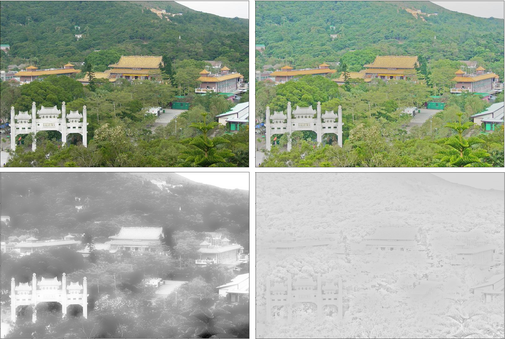
(Clockwise from top-left) Original Image, Contrast Reduced Image, Detail Layer, Base Layer

Note that the base layer is the only one that is filtered, this is what preserves the high frequency details in the HDR image. In the image above, note how the detail layer encodes the edge information of our original image. We can now construct the reduced contrast image by a simple gamma correction operation applied to the base layer and adding the result to the detail layer.

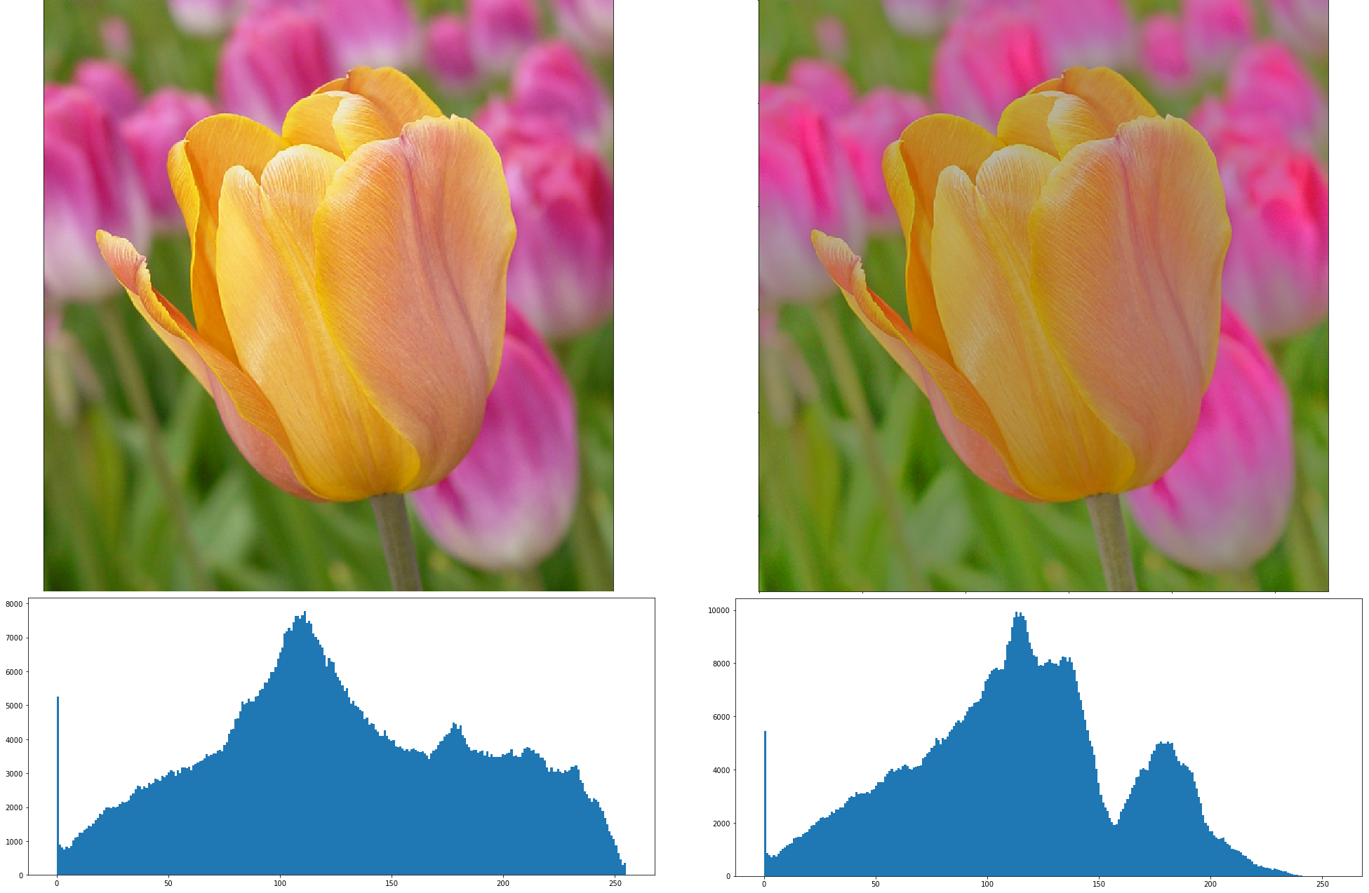
Let’s visualize an example with its histogram. The histogram illustrates that the bilateral filter compresses the range of pixel intensities in the image which leads to contrast reduction.

(Clockwise from top-left) Original image, Contrast reduced image, Histogram of contrast reduced image, Histogram of original image

[Github]

References

[1] Frédo Durand, Julie Dorsey - Fast Bilateral Filtering for the Display of High-Dynamic-Range