Generation of Images via Attribute Manipulation using Disentangled Representation Learning

22 Feb 2020

Disentangled representation learning studies how a problem can be broken into its constituent components which represent some underlying structure. This aids interpretability of representations learned by deep learning models and allows flexibility in sampling data from generative distributions. In this project, we’ll discuss how the paper on InfoGAN [1] modifies the GAN objective to learn these representations using an information theoretic framework.

The Sampling Problem

Let’s motivate a simple reason behind using representation learning. Suppose we want to train an agent to drive a vehicle in the city. A deep learning based algorithm might require a large amount of data; the process of recording and driving a vehicle to accumulate days of information is time-consuming and expensive. If it were possible to model the distribution of streets scenes and generate them synthetically instead we could generate voluminous samples of near-realistic data to train the agent. Greater flexibility could be added to the model if we could adjust the kind of samples generated by altering certain parameters in the model to generate, perhaps, scenes of one-way roads with no pedestrains. Disentangled representation learning will help us do just that. What’s more, this aids the interpretability of features learned by the model.

What is a Disentangled Representation?

While there is no formally agreed upon definition, [2] proposes a framework to characterize disentangled representations as a set of transformations that alter some properties of the underlying structure of the world without affecting its other properties. These properties may or may not be independent of each other, so it would be ideal to find base properties that are, in a sense, orthogonal to each other. For instance, we can’t keep a person’s face unchanged by altering their mouth but we can independently alter their mouth and eyes. So, it would be beneficial to use the properties of the nose and eyes as a latent feature to guide generation of face samples.

Formally, we would like to sample $X$ from a learned generative distribution $P_g$ that approximates some real world distribution $P_x$, given certain latent variables $Y$. From an information theoretic perspective, having information about these variables reduces our uncertainty about $X$. In other words, there is some mutual information between the variables $X$ and $Y$. Mathematically, mutual information is given as, \begin{equation} I(X; Y) = H(X) − H(X \vert Y), \end{equation} where $H(X)$ denotes the entropy of $X$ and $H(X \vert Y)$ is the conditional-entropy of $X$ given $Y$ ([3] is a really good resource for an intuitive and visual explanation of entropy.). We can view this as the information we gain about variable $X$ if $Y$ is observed. Now, if $Y$ had no information to give about $X$ (that is, $X$ and $Y$ are independent) then $H(X \vert Y) = H(X)$. Conversely, if $Y$ did have an influence then observing it would the reduce our uncertainty about $X$.

Learning a Distribution

These representations can be learnt jointly by also learning the distribution of our data. This is done via a Generative Adversarial Network (GAN). GANs are used for training a model to learn the distribution of the observed data and generate samples from this distribution. They consist of two players, one is the discriminator and the other is the generator. The generator tries to generate ‘fake’ examples which it wants to pass off as real, while the discriminator tries to distinguish between real examples and those from the generator by classifying them as either ‘real’ or ‘fake’.

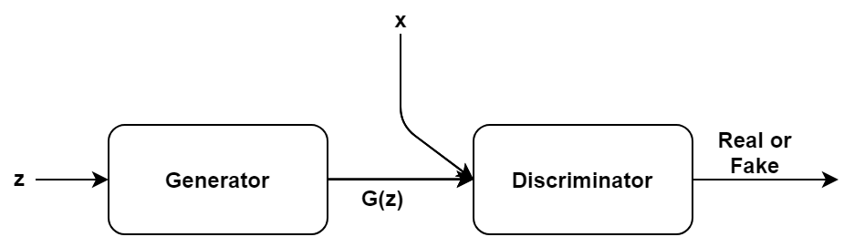
Within the context of deep learning, both players are modelled as deep neural networks. The generator samples from some noise distribution $z \sim Z$ and uses this noise sample to generate an example $G(z)$. During the training process the generator tries to generate better examples while the discriminator tries to get better at discriminating the ‘real’ examples (denoted by $x$) from the ‘fake’ ones (denoted by $G(z)$). The discriminator outputs $D(u), \, u = \{x, G(z)\}$, which is the probability of $u$ being fake (0) or real (1) and so behaves as a binary classifier. This game reaches an equilibrium when the generator becomes so good at generating examples that the discriminator can no longer distinguish between the ‘real’ and ‘fake’ examples. Ideally, of course, $P_g = P_x$ after the training process. Formally, the GAN objective is given by, \begin{equation} \min_G\max_D V(D,G) = \min_G\max_D E_{x \sim P_x} [log D(x)] + E_{z \sim P_z}[log (1 - D(G(z)))] \end{equation} [4] and [5] are good primers on GANs and the derivation of its objective function.

Latent Codes and the Information Regularized GAN objective

The generator doesn’t quite associate the dimensions of the noise $z$ to any semantically relevant features of the data it produces. Take the MNIST dataset, if the generator could assign the digit’s numerical value to some latent (hidden) variable then it would be possible to decompose the problem of generating digits to a simpler domain. It’s these latent variables that represent the disentangled representations of our digit data.

*Here the latent code varies as the rows of the picture. $c = 0$ is the first row in the image and the network associates the digit 5 with it.*

Here’s the crucial idea, we’d like to maximize the information we have about these latent codes (denoted by $c$) by observing the generated digits. This means that $I(c; G(z,c))$ should be high. [1] summarizes this formulation succinctly - given some sample from the generator distribution $x \sim P_G(x)$ we would like $P_G(c \vert x)$ to have small entropy ($H(X \vert Y)$). Equation (2) is then modified to incorporate the mutal information term as, \begin{equation} \min_G\max_D V_I(D,G) = \min_G\max_D V(D,G) - \lambda I(c; G(z,c)) \end{equation} To give better insight about the new objective function let’s go back to example with the MNIST dataset. If our generator operates on $z$ and $c$ to output a digit then through $c$ it can determine which digit should be generated. For instance, if $c = 4$, then the GAN could generate the digit 4. (Although, it should be noted that the digit’s numerical value and the value $c$ takes may not be the same but the correspondence is one-to-one. That is, once trained, a generator would associate, say, digit 9 with $c = 5$). It can then map $z$ to different “writing styles” of 4. The generator can thus use the information from the latent codes during the generation process.

Simplifying the Objective

The modified GAN objective is hard to optimize directly so we use the evidence lower bound or ELBO [6] to minimize some distribution $Q(c \vert x)$ which approximates $P(c \vert x)$. This lower bound is denoted by $L_I(Q, G)$. The auxiliary distribution $Q$ is parameterized by a neural network so in the implementation the objective that is minimized is,

\begin{equation} \min_{G,Q}\max_D V_I(D,G) = \min_G\max_D V(D,G) - \lambda L_I(Q, G) \end{equation}

[1] implements a DCGAN (deep convolutional GAN) and trains with this modified objective. The discriminator, $D$, and auxiliary distribution, $Q$, share all but the final convolutional layer. For $Q$ the final layer is a fully-connected layer that outputs either categorical variables (if $c$ is a discrete distribution) or parameters that describe a continuous distribution (like the mean and variance if $c$ is a Gaussian random variable). We can use softmax to compute the categorical loss and log-likehood loss for continuous random variables.

Experiments

We can always assign an appropriate prior to the latent codes. For simplicity, continuous latent codes are generally represented as a Gaussian random variable. Let’s analyse results from two datasets - MNIST and FashionMNIST.

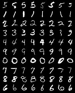
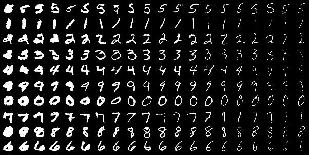
Let’s start with three latent codes for MNIST. In order to observe the impact of $C_1$, a categorical random variable, we fix the other two and vary $C_1 = \{0, 1, 2,…, 9\}$. From the image in section “Latent Codes” note how changing $C_1$, which encodes the digit type, changes the digit being generated.

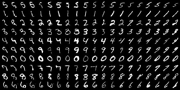
$C_2$ and $C_3$ are continuous random variables parameterized as Gaussian random variables. The images below show that $C_2$ alters the angular tilt of the digits and $C_3$ changes the thickness of the digits.

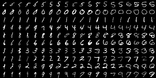
*As $C_2$ is varied between $[-2, 2]$ note how the digits tilt from left to right.*

*With $C_3 \in [-3, 3]$ notice how the thickness of the strokes changes from really thick to almost non-existent.*

With four latent codes for the MNIST dataset, $C_1$ is still defined as a categorical variable so it still encodes the numerical value of the digit. However, now $C_2$ varies the “writing style” of the digit 4.

*$C_2$ for MNIST with four latent variables alters the style of the digit 4.*

$C_3$ alters the area of holes in the digits. While $C_4$ now encodes the thickness of digits.

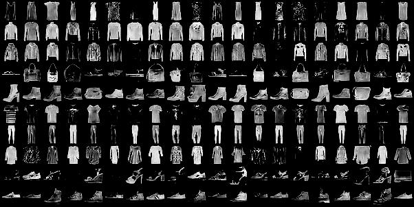
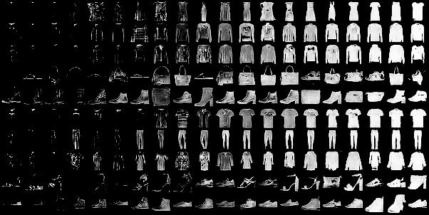
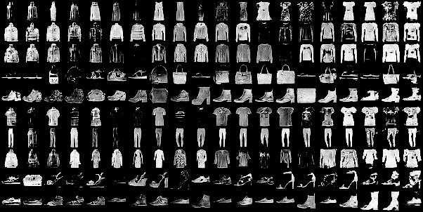
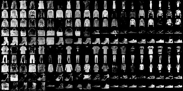
*$C_3$ for MNIST with four latent variables alters the area of holes.*

The results with the FashionMNIST dataset are even more interesting. This is modelled with four latent random variables ($C_1$ is categorical and the rest are continuous) and their effects are shown in the images below.